|
Overview
| This model illustrates the two main benefits of aggregating demand:
reduction in peak capacity requirements as well as increase in utilization. The increase in utilization comes about in two ways.
One is that the same demand is served by a smaller-sized pro forma capacity, but the second is that aggregation of random variables preserves
absolute variance, but reduces relative variance. The so-called "coefficient of variation" is a measure of variability relative to the mean, and this is
reduced as more and more random variables are summed.
In a cloud or utility environment, this is one of the drivers of service provider economics.
|
|
Basic Flow
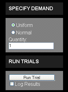
| First, select the distribution -- uniform or normal -- and the quantity of
random variables to be summed.
Second, run a random trial. Each trial generates 20 samples.
Third, view the results graphically. If the results are logged, they also can be viewed in tabular form.
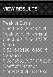
Fourth, review the key stats from the trial, such as mean, variance, and coefficient of variation.
Lastly, export the logged results from one or more trials to a spreadsheet with further analysis or charting capability.
|
|
Select Demand
|
Either uniform or normal demand may be selected as the underlying distribution, together with the number of random variables to be summed. The uniform distribution
is on the interval (0,1), and therefore has mean .5 and variance 1/12. The normal distribution has the same mean and underlying variance, but is truncated to be on the same interval,
which reduces the variance slightly (by clipping the long tails).

|
|
Run Monte Carlo Trials
|
Pressing the "Run Trial" button runs a trial with 20 sample results. Each result is the sum of n randomly generated numbers, where n is the quantity specified.
|
|
View Results Graphically
|

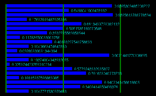
The results of each trial are shown graphically on a bar chart, which is normalized to be between 0% and 100% of the pro-forma peak. For example, suppose that 20 variables are summed. Since each of the results ("determinations") of each
variable lie between zero and one, this sum will lie between zero and twenty.
By increasing the quantity, and running a trial, it will be seen that the results, which start out spread widely, become closer and closer to each other.
|
|
View Statistics
|

View the statistics generated from the trial. |
|
Export Data for Analysis
|
By selecting the raw data in the results log and using CTRL-C to copy the data, it may then be pasted into a spreadsheet tool for further data analysis
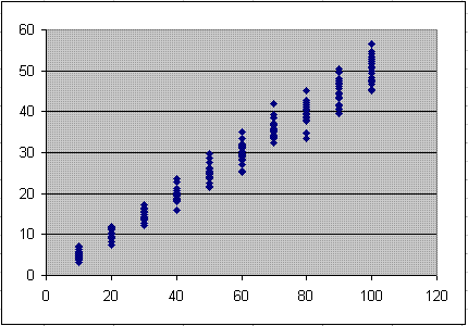
and custom charting. Using columns one and two provides the raw (unnormalized data) to feed a scatter plot such as shown below, demonstrating the trend line that
the peak drops off as the number of demand curves being aggregated increases.

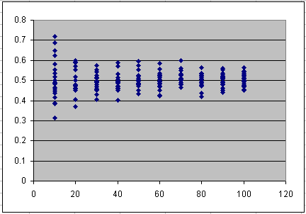
Using columns three and four of the table provides the normalized data, which is the raw data divided by the quantity of variables. This shows that the relative spread (the coefficient of variation, which is the standard deviation divided by the mean)
also drops off. For the uniform distribution, it actually drops off as the square root of the number of variables summed, as can be seen in the diagram.

|
|
About
|
This model was written by Joe Weinman in about 300 lines of code,
which are a mixture mostly of HTML and JavaScript, using Microsoft Visual Web Developer 2008.
It has been tested in Firefox 2.0 (Mozilla 5), Safari 3.1, and Internet Explorer 7.0. It even runs on an iPhone 3G, at about the same speed as on a laptop, even though most computation is performed on the client.
|
|
