Second, the resulting demand curve may be viewed in either the Annual or Weekly Demand windows. The Weekly Demand window is a bar chart of every single hour of a one week period. The Annual Demand window shows the maximum, minimum, and or average hourly demand for each of the 365 days in the year.
Third, a variety of capacity strategies may be tried. By allowing additions and reductions to capacity, it may be possible to reduce the expenses associated with fixed capacity. The challenge is that too little capacity may lead to some demand not being served, which has a financial penalty associated with it. And, changing capacity may incur charges.
Fourth, cost assumptions may be modified. Whether costs for fixed capacity, costs for capacity modifications (installs or decommissioning), opportunity costs of unserved demand, or costs for utility servers.
Fifth, statistics may be viewed, e.g., minimum demand, average demand, unserved demand hours.
Lastly, the relative costs and underlying drivers of four different types of architectures / business models may be viewed as a bar chart.
|
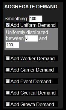
The demand shaping window is used to characterize the nature of the demand. Each demand type
has different parameters that may be used to shape the curve. For example, the cyclical demand
type has controls to adjust amplitude (maximum number of servers), period (time it takes for the
cycle to repeat itself), and offset (shifting the peak of the cycle forward or backward in time).
Checkboxes indicate whether the demand is to be included in the analysis or not. Finally, the
smoothing parameter at the top of the window may be used to smooth demand. It specifies the maximum change
(delta) in any time period. Lower numbers smooth demand, whereas higher numbers may
leave it more jittery.
Uniform Demand -- Uniformly distributed between min servers and max servers. Worker Demand -- 0 after hours, but uniformly distributed weekdays from 9 to 5. Gamer Demand -- Gamers are assumed to have day jobs, but are active nights and weekends. Event Demand -- Used to model special events, e.g., concerts, disasters, movie premieres. The parameters specify the typical duration of the events, the typical time between the end of an event and the start of the next, and of course the minimum and maximum demand. "Typical" times are averages, and durations may vary from 50% to 150% of the specified duration. Cyclical Demand -- For daily, weekly, monthly, quarterly, or annual cycles. Growth Demand -- Starts the year within a particular min / max range, and is smoothly interpolated to a different min / max range. This can also be used to model declines, or even a change in variance (e.g., the year may start with demand in the range from 0 to 100, but end with a more compressed range, say, 40 to 60. |
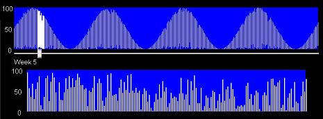
The annual and weekly demand may be viewed. Clicking on a daily demand bar or entering a week number changes the week that is "zoomed in." Hovering over a demand bar shows the time slot and information associated with it. Hovering over the blue capacity graph shows the capacity level and the duration it is in effect.
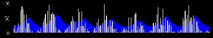
A variety of capacity strategies may be attempted. The initial capacity and minimum capacity may be adjusted. Capacity increases may be allowed, based on recent peak, average, or minimum demand values. Delay times for placing the capacity "order" may be adjusted. Separately, capacity decreases may be similarly allowed. However, there are costs associated with having capacity (in effect, monthly lease costs or depreciation), capacity increases (installation and turn-up), or capacity decreases (e.g., transportation, removal, reconditioning). Different types of demand curves may be more or less amenable to different capacity strategies. Flat demand, with little variance (min close to max) can effectively be supported by a fixed capacity strategy. Steady growth can be amenable to relatively infrequent upgrades which may be planned in advance. Cyclical requirements can be met by alternating increases and decreases. However, trying to rapidly respond to random demand changes, like buying stocks after an up day in the market and selling them after a down day can be counterproductive. If response time is too slow, capacity may be being decreased after demand has begun to increase. And, trying to follow every twist and turn in the demand curve can cause churning of the capacity, incurring excessive charges.
A variety of statistics are automatically generated each time any assumptions or inputs change. These include things like the maximum demand, the minimum demand, the average demand, and how many unit-hours of demand would be unserved due to capacity shortfalls. Also, total charges are displayed for four different models.
A pure pro forma fixed capacity model. This assumes unvarying capacity as high as peak demand.
A variable capacity model, with either capacity increases, decreases or both. Deltas may save capacity costs, but also run the danger of creating additional cost through unserved demand.
A pure utility model. The capacity model (fixed or variable) is ignored, and unbounded resources are assumed to be available in the cloud, but a premium is paid for each unit-hour of capacity.
A hybrid model. Capacity as specified is used and charges incurred, AND utility resources are leveraged to ensure that there is no unserved demand.
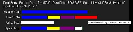
The pure pro forma fixed capacity model, the variable capacity model, the pure utility model, and the hybrid model are displayed graphically so that they may be compared. Adjusting capacity strategies, demand curves, and/or cost assumptions alter the relative costs.